Krizhevsky, Sutskever, Hinton and ImageNet
Introduction
In this post, we will cover and briefly summarize the article titled ImageNet Classification with Deep Convolutional Neural Networks authored by Alex Krizhevsky, Ilya Sutskever, and Geoffrey E. Hinton of the University of Toronto and published in Advances in Neural Information Processing Systems 25 (NIPS 2012). The official abbreviation for the conference changed from NIPS to NeurIPS in 2018. NeurIPS is a machine learning and computational neuroscience conference held every December since 1987.

The article describes the architecture and training of a deep convolutional neural network to classify the 1.2 million high-resolution images of the ImageNet LSVRC-2010 contest into the 1000 different classes. ImageNet is an ongoing research effort to provide researchers an easily accessible image database. As an organization, it annually (2010–2017) held The ImageNet Large Scale Visual Recognition Challenge (ILSVRC). This research competition evaluates algorithms for large scale object detection and image classification.
Procedures
The dataset used for the ILSVRC-2010 competition and hence the object of the article is a subset of ImageNet with close to 1000 images in each of 1000 categories. The dataset adds up to about 1.2 million training images, 50,000 validation images, and 150,000 testing images. The University of Toronto team trained the network on the (centered) raw RGB values of the images’ pixels.
The metrics used to assess the model performance were top-1 and top-5, where the top-5 error rate is the fraction of test images for which the correct label is not among the five labels considered most probable by the model.
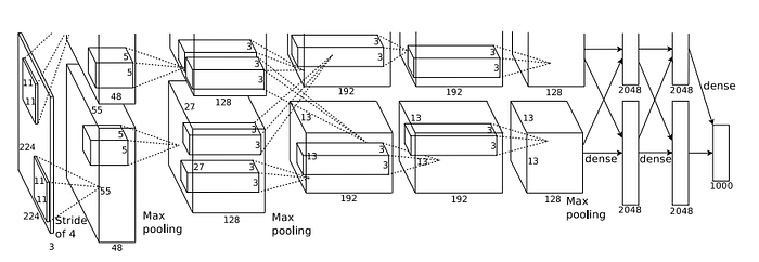
The Deep Convolutional Neural Network contains eight learned layers. The first five are convolutional and the remaining three are fully-connected. The output of the last fully-connected layer is fed to a 1000-way softmax which produces a distribution over the 1000 class labels. See the image below for a depiction of the architecture.

Results
Besides the anecdotical value of the story about winning the competition, the article provides insight and explanations about the chosen architecture and its performance. They address four different engineering choices. Here is the list in decreasing relevance:
- ReLU Nonlinearity
- Training on Multiple GPUs
- Local Response Normalization
- Overlapping Pooling
The article shows how the use of the ReLu Nonlinearity greatly busts performance in comparison to the traditionally used sigmoid or tanh activation functions.
To address the Overfitting problematic the researchers used both Data Augmentation and at the time of the article newly introduced Dropout technique. They trained the models using stochastic gradient descent with a batch size of 128 examples, a momentum of 0.9, and a weight decay of 0.0005. The Network took between five and six days to train on two GTX 580 3GB GPUs.
The architecture choice and the use of separate GPUs led to a specialization in the learning accomplish by each unit. One GPU learned features were mainly color agnostic and the other color-specific.
Conclusion
The overall performance (top-1 and top-5) may not seem too impressive today after 10 years. But it is important to bear in mind that it represented a two-digit improvement in comparison to what it was considered state of the art at the time.
Top-1
Berg Et al. (Sparse coding) 47.1%;
Sánchez Et al. (SIFT + FVs) 45.7%;
Krizhevsky Et al. 37.5%
Top-5
Sparse coding 28.2%;
SIFT + FVs 25.7%
Krizhevsky Et al.17.0%

The researcher clearly stated:
“All of our experiments suggest that our results can be improved simply by waiting for faster GPUs and bigger datasets to become available.”
The ML community did not have to wait long for these foreseeable improvements. Today’s flagship GPU from Nvidia is the GEFORCE GTX 1080 Ti 11 GB, which has almost 4 times more memory than its ancestor the GTX 580 3GB, used for the present study. Memory is only one aspect, but there are countless other advancements in both hardware and software. The size and availability of Datasets have also increased dramatically, social media and IoT devices have become a continuous source of data.
Personal Notes
Reviewing this kind of historical articles always give a perspective on the path that bought us to where we are now. It never stops to amaze me, how little time, only a decade, has elapsed since the introduction of concepts and practices such as ReLu, parallel processing, and Dropout that are considered standard today.

Only a little more than a decade before Krizhevsky the LeNet-5 by LeCunn Et al. with its paper Gradient-Based Learning Applied to Document Recognition (LeNet-5) made its debut (see Figure). Today we are talking about the YOLO v5 released only weeks after its predecessor the YOLO v4.

This impressive pace leaves me with the somehow disturbing and exciting question:
Who knows where we will be 10 years from now?